Example analysis

CHESS has two typical use-cases, which are showcased in the Publication:

1. Finding genomic regions with differences in their chromatin conformation between two samples. This is useful for example for the identification of disease driving changes.
2. Comparing the chromatin conformation between two distinct regions in the same or in different genomes. This is useful for example for quantifying the grade of conservation of chromatin conformation in evolution.

Finding differences between samples of different conditions

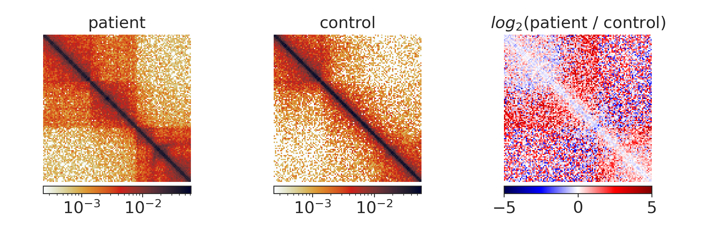
This example illustrates how CHESS can help to identify genomic regions that differ in their chromatin conformation between two samples, by the example of samples from a DLBCL <https://en.wikipedia.org/wiki/Diffuse_large_B-cell_lymphoma> patient and a control person. The analysis of these data is also showcased in the CHESS paper, Figure 5.

For this analysis, we will need only three input files for CHESS:

1. Balanced Hi-C data for the first sample
2. Balanced Hi-C data for the second sample
3. The coordinates of the regions that should be compared in bedpe format.

1. and 2. can be in Juicer, Cooler or FANC format. However, we advice to use Juicer of FANC files for performance reasons.

3. should be supplied in BEDPE format.

If we want to scan a whole chromosome or genome for differences, we can use the chess pairs subcommand to generate the 3. input file.

To follow along with the example analysis, first move to the data location:

cd examples/dlbcl

Generating a pairs input file

In this example analysis, we will search the entire chromosome 2 for differences. For this, we first need to generate the pairs file with the chess pairs subcommand. We will compare regions of 3 Mb size with a step size of 100 kb. In addition, chess pairs needs to know the sizes of the chromosomes for which we want to generate the pairs. Here we supply ‘hg38’ as an genome identifier:

chess pairs hg38 3000000 100000 \
./hg38_chr2_3mb_win_100kb_step.bed --chromosome chr2

Running the search

With all necessary input files prepared, we can run the search with the chess sim subcommand:

chess sim \
ukm_control_fixed_le_25kb_chr2.hic \
ukm_patient_fixed_le_25kb_chr2.hic \
hg38_chr2_3mb_win_100kb_step.bed \
ukm_chr2_3mb_control_vs_patient_chess_results.tsv

The output data are stored in the ukm_chr2_3mb_control_vs_patient_chess_results.tsv file.

Inspecting the results

To inspect which regions show differences between the two samples, it is useful to first inspect the similarity index along the compared chromosome. Aside from the calculated similarity index, the signal-to-noise ratio is important. One way to display this information together is this (please check out the jupyter notebook at examples/dlbcl/example_analysis.ipynb for the code to generate these plots and subset data):

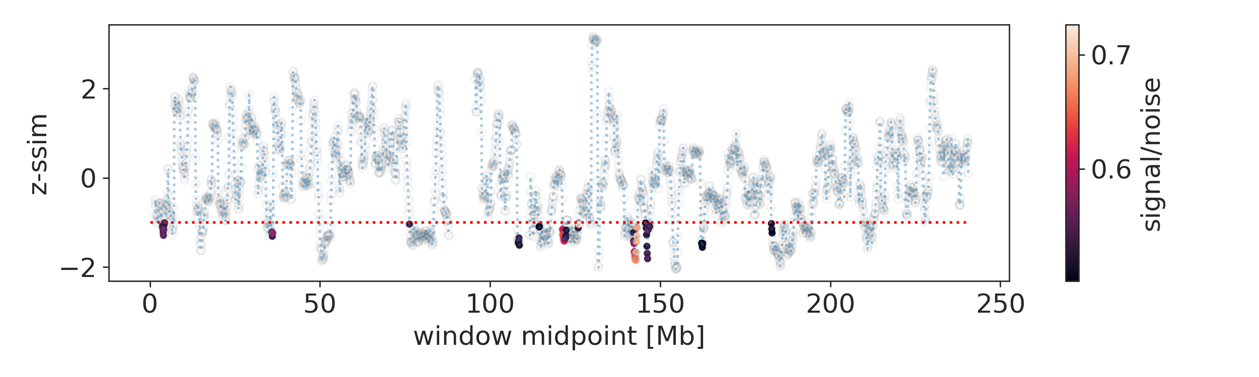
Here we display only regions with a signal-to-noise ration > 0.5 and a z-normalised similarity score < -1 as colored dots, the rest is gray. The most interesting regions are highlighted by deep dips with above threshold signal-to-noise ratios, for example the region around 148 Mb:

Extracting features

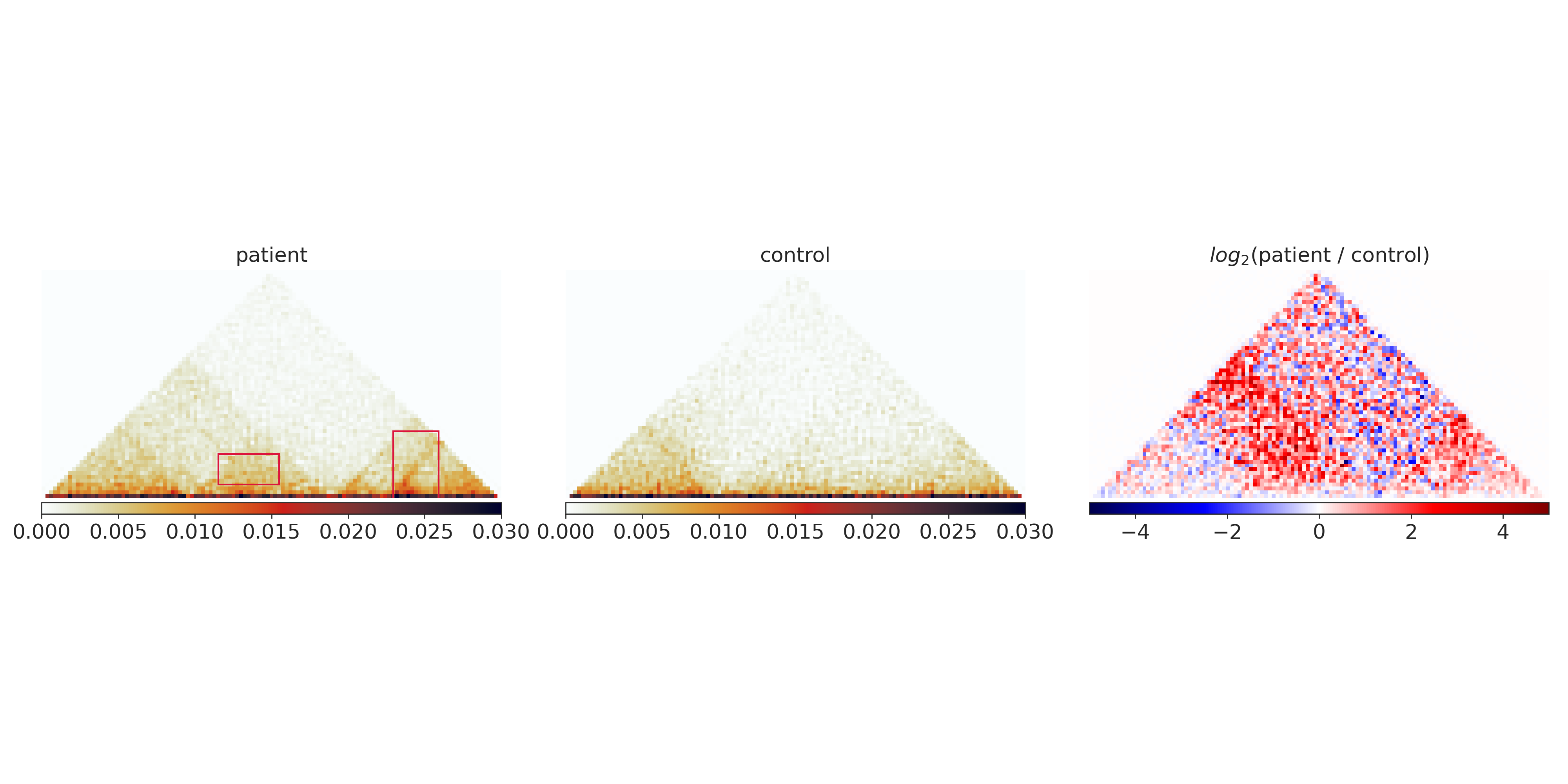
We now might want to highlight the features in these regions that show particularly strong differences. This can be done with the chess extract command. To use it, we first need to decide on a subset of regions that contain strong differences, e.g. by filtering with the signal-to-noise > 0.5 and z-ssim < -1 cutoffs used above (see the jupyter notebook for subsetting code). We then prepare an output directory

mkdir features

and then run chess extract:

chess extract \
filtered_regions_chr2_3mb_100kb.tsv \
ukm_control_fixed_le_25kb_chr2.hic \
ukm_patient_fixed_le_25kb_chr2.hic \
./features

We are here using the command with default parameters. Please note that the input parameters have to be fine tuned depending on the size of the analyzed regions and the target features. For now, some experimentation by the user is required, but we are planning to release a guide to this in the future.

In our example region, the following parts are marked by the extraction algorithm in default mode, marking the differential TAD structures:

Classifying features

Finally, we can gain more information about the kind of features that we extracted in the previous step by grouping them by similarity of their topology. This can be done with the chess crosscorrelate command, which we can simply apply to the result files of the previous step. E.g. to classify the gained features, we run

chess crosscorrelate \
features/gained_features.tsv \
filtered_regions_chr2_3mb_1mb.tsv \
./features/

We obtain ./features/subregions_2_clusters_gained.tsv, where the 2 corresponds to the 2 clusters identified in this analysis. The results file has three columns: the cluster number, the region id and the feature id. Using the feature id column, each feature in the input file (features/gained_features.tsv) can be mapped to its class.

Choosing a window size

In this analysis, we compared windows of 3 Mb size between our samples. In general, choosing a different window size should be correlated, with large windows simply averaging over the effects observed in smaller windows.

Despite the correlation, different window sizes can yield different results in some regions:

• Larger windows cover more and longer long-range interactions:
  • If you are interested in changes of large effects stretching over long genomic distances, choose a larger window size.
  • However, long-range interactions tend to be more noisy. The larger the window size, the smaller the number of regions that will pass a given signal-to-noise threshold. If your analysis does not return any regions of strong dissimilarity above your signal-to-noise threshold, lower the threshold or try a smaller window size.
• The larger the window, the smaller the effect of small changes:
  • If you are interested in finding changes in single TAD boundaries, choose a small window. Large windows will cover multiple boundaries and the score of the window will reflect their combined change.